
Lottery formats differ in number field size, pick size, and whether an extra ball is part of the draw. Those three things determine how many total combinations a game can produce, which is what sets the probability tied to each ticket.
This article examines how probability and combinatorics describe lottery game structure — and what the math cannot do.
Table of Contents
How Number Field Size and Pick Size Shape Lottery Probability
Two things control how many total combinations a lottery can generate: the size of the number field and the pick size.
A drum with 42 balls produces fewer possible outcomes than one with 49. A Pick-5 game creates fewer combinations than a Pick-6. Fewer combinations mean a higher probability per ticket — though that still doesn’t make winning likely in any absolute sense.
The Impact of the Extra Ball on Probability
Many lotteries include an extra ball. It gets called different things — Powerball in Powerball, Lucky Star in EuroMillions — but the math depends on one thing: where it comes from.
When supplementary numbers come from the same pool as the main draw, as in TattsLotto and the Irish Lotto, they only affect lower-tier prizes. The jackpot probability doesn’t change — it’s still determined by the primary drawn numbers alone.
When the extra ball is drawn from a separate pool, the total sample space expands. Winning the jackpot now means matching both the main numbers and that additional ball, which lowers the probability of hitting the top prize. These formats tend to offer more prize tiers and more frequent smaller wins — but reaching the jackpot gets harder.
Several U.S. state lotteries skip the separate extra-ball pool entirely.
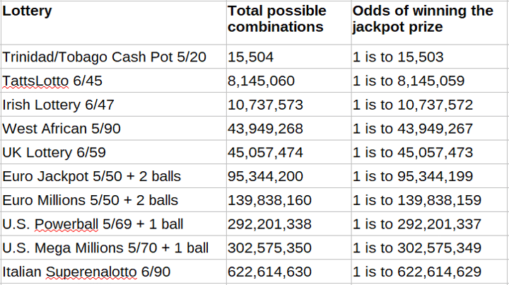
The table below compares jackpot odds across selected formats, showing how game structure shapes the total combination count.
The Statistical Reality
Probability runs from 0 to 1. Zero means impossible. One means certain. No ticket for a specific draw means the probability of winning that jackpot is exactly zero — full stop.
Lottery odds are sometimes compared to rare events like shark attacks to make the numbers feel graspable. Those comparisons can help with intuition, but they change nothing. The probability of winning a lottery jackpot stays extremely low and fully independent in every draw, however you frame it.1,2
The table below shows selected U.S. state lottery games and their jackpot probabilities.
| LOTTERY GAME | PROBABILITY |
|---|---|
| Match 4 (WA) | 1 in 10,626 |
| Big Sky Bonus (MT) | 1 in 31,465 |
| Lucky Lines (OR) | 1 in 65,536 |
| Treasure Hunt (PA) | 1 in 142,506 |
| North 5 (MN) | 1 in 169,911 |
| Badger 5 (WI) | 1 in 169,911 |
| Cash 25 (WV) | 1 in 177,100 |
| Cash 5 (CO) | 1 in 201,376 |
| Weekly Grand (ID) | 1 in 201,376 |
| Cash5 (CT) | 1 in 324,632 |
| Match 5 (MS) | 1 in 324,632 |
| Dakota Cash (SD) | 1 in 324,632 |
| Cash Five (TX) | 1 in 324,632 |
| Fantasy 5 Midday/Evening (FL) | 1 in 376,992 |
| Cash 5 (OK) | 1 in 376,992 |
| Easy 5 (LA) | 1 in 435,897 |
| Roadrunner Cash (NM) | 1 in 435,897 |
| Wild Money (RI) | 1 in 501,942 |
| Palmetto Cash 5 (SC) | 1 in 501,942 |
| Daily Tennessee Jackpot (TN) | 1 in 501,942 |
| Natural State Jackpot (AR) | 1 in 575,757 |
| Fantasy 5 (CA) | 1 in 575,757 |
| Kentucky 5 (KY) | 1 in 575,757 |
| Gimme 5 (ME) | 1 in 575,757 |
| Bonus Match 5 (MD) | 1 in 575,757 |
| Fantasy 5 (MI) | 1 in 575,757 |
| Show Me Cash (MO) | 1 in 575,757 |
| Gimme 5 (NH) | 1 in 575,757 |
| Take 5 Midday/Evening (NY) | 1 in 575,757 |
| Rolling Cash 5 (OH) | 1 in 575,757 |
| Gimme 5 (VT) | 1 in 575,757 |
| 5 Star Draw (ID) | 1 in 610,880 |
| Idaho Cash (ID) | 1 in 610,880 |
| Montana Cash (MT) | 1 in 610,880 |
| Cowboy Draw (WY) | 1 in 610,880 |
| Pick 5 (NE) | 1 in 658,008 |
| Fantasy 5 (AZ) | 1 in 749,398 |
| Fantasy 5 (GA) | 1 in 850,668 |
| Hit 5 (WA) | 1 in 851,000 |
| Cash 5 (NC) | 1 in 962,598 |
| Cash 5 (PA) | 1 in 962,598 |
| Lucky Day Lotto Midday/Evening (IL) | 1 in 1,221,759 |
| Ca$h 5 (IN) | 1 in 1,221,759 |
| Jersey Cash 5 (NJ) | 1 in 1,221,759 |
| Cash 5 (VA) | 1 in 1,221,759 |
| Cash Ball 225 (KY) | 1 in 1,309,000 |
| Win for Life (OR) | 1 in 1,353,275 |
| Gopher 5 (MN) | 1 in 1,533,939 |
| Multi-Win Lotto (DE) | 1 in 1,623,160 |
| Tennessee Cash (TN) | 1 in 1,623,160 |
| SuperCash! (WI) | 1 in 1,631,312 |
| Texas Two Step (TX) | 1 in 1,832,600 |
| Multi-Match (MD) | 1 in 2,032,151.70 |
| Super Kansas Cash (KS) | 1 in 2,517,200 |
| Jackpot Triple Play (FL) | 1 in 3,122,273.33 |
| Loto Cash (PR) | 1 in 3,246,320 |
| Revanchax2 (PR) | 1 in 3,246,320 |
| Lotto (MO) | 1 in 3,529,526 |
| Arkansas Lotto (AR) | 1 in 3,838,380 |
| Colorado Lotto+ (CO) | 1 in 3,838,380 |
| Bank a Million (VA) | 1 in 3,838,380 |
What a Math-First Look at Lottery Games Actually Examines
Most mathematicians don’t play the lottery. Some do, and their approaches occasionally surface in the public record.3,4
What probability-based game analysis actually looks at comes down to a few structural factors.
1. The Total Number of Combinations (Sample Space)
The sample space — the total number of possible combinations — is the single most important structural factor in comparing games. If Game A has odds of 1 in 40,000 and Game B sits at 1 in 14,000,000, Game A has a higher probability per ticket because fewer combinations exist. That is a structural comparison. It is not a guarantee of anything.
2. Prize Structure Relative to Odds Distribution
Some games concentrate nearly all prize value in a single jackpot. Others distribute it across several tiers. A probability-based view of both reveals whether a game places most of its weight on rare large wins or more frequent small ones. No lottery has positive expected value over the long run. This analysis describes risk distribution within the game’s design, not a path to profit.
3. Historical Data as a Randomness Check
Some people go through past results looking for clues about future draws. That’s not how a random process works. A different use of historical data is to verify that the draw process is genuinely random — if the outcome distribution tracks with what probability theory predicts over many draws, that confirms the draw mechanism is functioning correctly. Past draws have nothing to say about future ones.
To study how truly random lottery numbers distribute across draws, I built a PHP simulation in March 2020 using PHP’s random_int() function — cryptographically secure random integer generation. The simulation generates large volumes of lottery-style combinations and plots each result on a grid, making visible how a genuine random process distributes outcomes over many trials. You can read more about that work at Random Lottery Numbers: A Study of Long-Run Statistical Behavior.
4. Draw Frequency and Budget
Playing more draws does not change the probability on any single ticket. It increases exposure to the same underlying risk. The expected value of each individual play stays the same regardless of how many times someone participates.
5. Expected Value — What It Actually Means
Most lottery games are designed so the average player loses money over time. Expected value analysis makes that reality explicit. Randomness governs outcomes. No selection method changes the expected value of any lottery ticket.
6. Regulation and Transparency
Every game worth analyzing has published odds, clear rules, and recognized regulatory oversight. Without verifiable data, probability-based evaluation is impossible. Transparency is where honest analysis has to begin.
Examining Lottery Games Through the Lotterycodex Framework
The Lotterycodex framework examines the math behind each game’s structure. Every lottery runs within a defined probability structure. Outcomes are always random and independent — but that structure can still be analyzed using combinatorics and probability theory to describe how different combinations are distributed across the outcome space, not to forecast results.
1. Single-Matrix Games and Combinatorial Transparency
Games built around a single number field produce a combination space that comes entirely from one source. Pick-5 from 1–50, Pick-6 from 1–49 — the full sample space is calculable from a single binomial coefficient. Add a bonus ball from a separate pool and the probability structure layers up: the total outcome space now assembles from multiple components, which changes the calculation and makes the actual odds less immediately transparent.


Within the Lotterycodex framework, I focus the combinatorial analysis on the main number matrix. The bonus ball operates outside the primary combinatorial structure being examined.
2. The Distribution of Combinatorial Compositions
Every combination carries the same probability of being drawn in a single draw. But group all combinations by their combinatorial composition and those groups are not equal in size. Some hold far more combinations than others. Under the law of large numbers — which describes how observed frequencies converge toward theoretical probabilities as the number of trials grows, not how any single draw behaves — larger groups appear more often across many draws, simply because more of the total outcome space belongs to them.
The Lotterycodex framework sorts these groups into four categories: Prevalent, Occasional, Rare, and Extremely Rare. These labels reflect how often certain combinatorial composition types are expected to show up over very large numbers of draws, based on combinatorial mathematics alone — not forecasting or prediction of any kind.
I developed these classifications through independent research starting in 2017, building the framework as a descriptive and educational model — a way to study how different combinatorial compositions are distributed under probability theory, not a method for predicting or controlling outcomes. In a 5/32 lottery, that breakdown includes roughly 4 Prevalent templates, 24 Occasional, 24 Rare, and 4 Extremely Rare.

In a 6/45 format, the split is roughly 6 Prevalent, 32 Occasional, 30 Rare, and 16 Extremely Rare.

These categories are tools for probability awareness and structural understanding. They do not imply control over outcomes or guarantee any result.
3. Frequency Ratio as a Long-Run Structural Reference
A frequency ratio describes how often a specific combinatorial composition is expected to appear across many draws, on average, under random conditions. It reflects how that compositional type sits within the full population of all possible combinations — and nothing beyond that.
In Lotterycodex, I use the term “frequency ratio” rather than “odds in favor” to describe this relationship. The word “odds” is commonly interpreted as odds of winning or losing — a framing that doesn’t apply when describing how often a combinatorial composition appears across many draws. A frequency ratio more precisely captures the statistical relationship: it describes long-run distribution, not prediction, not control, not any implied advantage for the player.

In a 7/50 game, the combination 1-2-3-4-5-6-7 belongs to a template with a long-run relative frequency of roughly 1 in 634 draws. Across a very large sample, that translates to about 3 appearances per 2,000 draws on average. These are statistical expectations under random sampling — not scheduled outcomes, not timing signals.
4. Law of Large Numbers Alignment in Historical Draw Data
Lotterycodex tracks major lottery games over time to show how real draw results gradually move toward their theoretical probability expectations — which is exactly what the law of large numbers describes in practice. The law of large numbers is a formal probability theorem about long-run convergence: as draws accumulate, observed relative frequencies tend toward their underlying theoretical probabilities. It says nothing about the outcome of any individual draw.

Green bars in the visualization show the theoretical expected frequency — what combinatorics and probability theory predict. Orange bars show what historical draws actually produced. Gaps between them are normal in any finite random sample. As the number of draws grows, the two tend to close in on each other. That is the law of large numbers at work. In any single draw, every individual combination still carries the same probability.

Occasional templates hold a smaller share of the total combination space compared to Prevalent ones, so they show up less often over the long run. Not because draws favor or avoid any particular composition — just because fewer combinations belong to those groups.


Rare and Extremely Rare templates represent groups with a thin slice of the total combination space. Because draws are random and uniform, groups with fewer total combinations will naturally surface less often over many draws. The green-versus-orange comparison makes that mathematically visible — for educational purposes only. No timing or prediction is implied.
What the Math Actually Settles
The math keeps landing on the same point: a smaller sample space produces a higher relative probability per ticket. A single-matrix game is easier to analyze than one with a separate extra ball layered on top. A game with published odds and recognized regulatory oversight can at least be evaluated honestly.
None of that changes what the lottery fundamentally is. These games carry negative expected value over the long run. No selection method predicts outcomes or overrides randomness. Every combination remains equally likely in any individual draw.
What the Lotterycodex framework provides is probability literacy — a clearer picture of how combinations are distributed across the total outcome space, and what that distribution means when you look at it over time. It is not a winning method. It is a mathematical description of what you are actually playing.
Understand Lottery Games Using Math-Based and Data-Driven Analysis
 Explore the Lotterycodex Calculator
References